What is CFD aerodynamic analysis?

The big picture of CFD analysis

CFD analysis is a method of computing airflow on a computer without conducting a physical wind-tunnel test. By numerically obtaining the pressure distribution, flow velocity and drag/lift coefficients around the vehicle, you can evaluate and improve aerodynamic performance before building an actual car.

The basic idea of CFD is simple. The space surrounding the vehicle is divided into extremely fine “cells,” and the fluid’s physical quantities (velocity, pressure, temperature, etc.) are computed in each cell. In external aerodynamic analysis of an automobile, this cell count reaches tens of millions to hundreds of millions. The finer the cells, the higher the accuracy — but the computational cost rises proportionally, so where to concentrate the mesh directly reflects the skill of the analysis design.

The governing equations ── the Navier-Stokes equations

What CFD solves are the Navier-Stokes equations. These are partial differential equations that describe the motion of a fluid — Newton’s second law of motion applied to fluids. They consist of three equations — conservation of mass (the continuity equation), conservation of momentum and conservation of energy — and describe the temporal and spatial changes of the fluid’s velocity and pressure fields.

These equations are nonlinear and have no analytical (closed-form) solution in the general case. The basic CFD strategy is therefore to discretize space into cells and obtain an approximate solution through iterative computation. Because turbulence dominates in automotive aerodynamics, the RANS (Reynolds-Averaged Navier-Stokes) approach — combined with turbulence models such as k-ω SST or Spalart-Allmaras — is widely used.

STEP 01 ── Pre-processing (mesh generation)

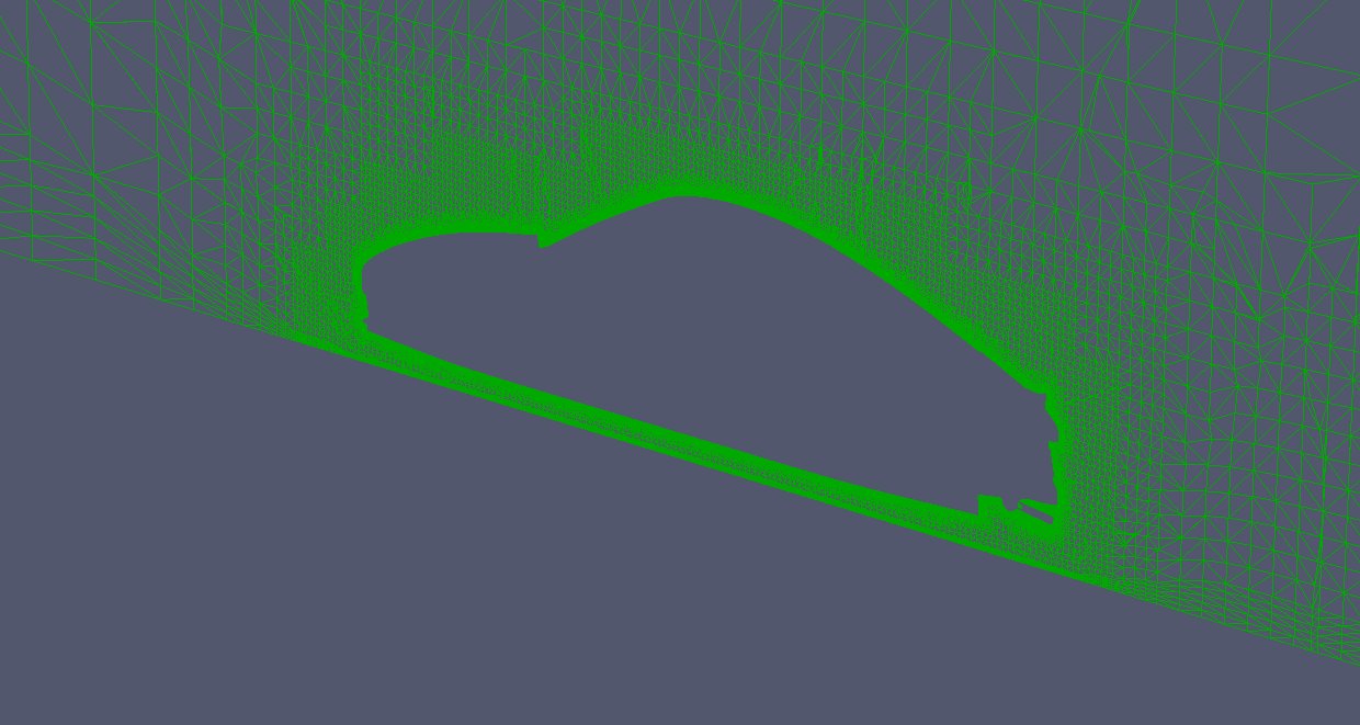
The first step of CFD analysis is pre-processing, where the mesh (grid) of the computational domain is created. The input is the vehicle’s geometry data — STP (STEP) files exported from CAD software such as CATIA, or STL (triangle mesh) files obtained from 3D scanning.

Because CAD data such as STP is defined by NURBS surfaces, we first tessellate it (convert it into a triangle mesh) so the CFD solver can handle it, creating a surface mesh. STL files are already in triangle-mesh form, so they can be used directly as the basis for the surface mesh.

Once the surface mesh is ready, the space around the vehicle is filled with a volume mesh. The spatial mesh is broadly divided into two types: the boundary-layer mesh and the volume mesh.

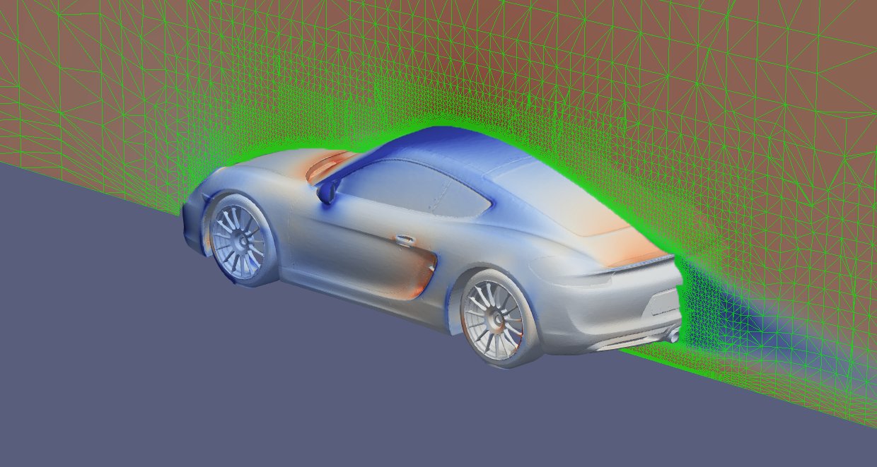
The boundary-layer mesh is a set of high-resolution cells arranged in thin layers along the body surface. Because flow velocity changes sharply near the wall (large velocity gradients), failing to resolve this region adequately significantly degrades the prediction accuracy of drag and downforce. Especially in the development of competition vehicles chasing aerodynamic performance, the quality of the boundary-layer mesh determines the analysis accuracy.

The volume mesh fills the cells outside the boundary layer, keeping the cell count down by enlarging the cell size with distance from the body. However, in regions of intense flow change — such as a wing’s wake or the vortex structures in the wheel houses — refinement (local subdivision) is applied to secure the necessary resolution.

STEP 02 ── Solver (running the computation)

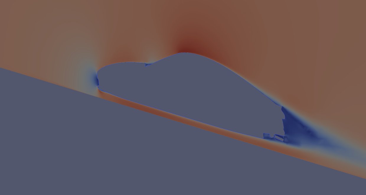
Once the mesh is complete, the solver computes the physical quantities in each cell. In external aerodynamic analysis of an automobile, the mesh count runs to tens of millions to hundreds of millions of cells. Solving a system of equations at this scale takes an impractical amount of time on an ordinary workstation, so a large-scale parallel computing environment is required.

We use an HPC (High Performance Computing) environment — what is commonly called a supercomputer. By running parallel computations on hundreds to thousands of cores, we can obtain results within a practical time even for analyses on the order of hundreds of millions of cells. This scalable computing environment lets us deliver high-accuracy analysis in a timely manner without compromising on mesh coarseness.

The solver iterates, converging the velocity, pressure, turbulence quantities and so on in each cell. Convergence is judged not only by monitoring the residuals but also by confirming the stability of physical quantities such as the drag and lift coefficients.

STEP 03 ── Post-processing (visualization and evaluation of results)

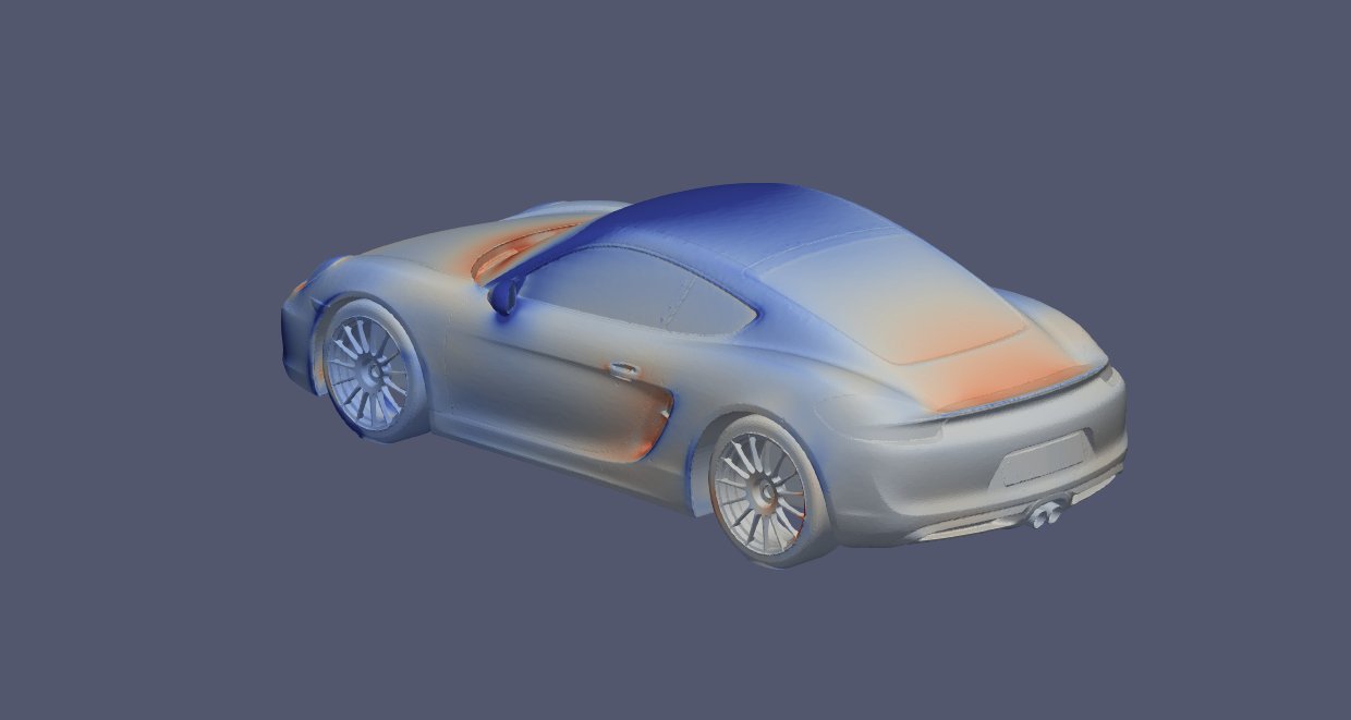
Once the solver computation is complete, we move on to post-processing, where the results are visualized and the aerodynamic performance is evaluated. In post-processing, the results are rendered using various techniques to visually grasp the flow at the locations whose performance needs to be assessed.

Typical visualization techniques include sectional contours (displaying velocity or pressure in color on an arbitrary section across the body), surface contours (mapping the pressure coefficient or skin friction onto the body surface) and streamlines (visualizing the trajectory of the airflow). In addition to this visual information, the loads acting on each region (drag, lift, moment) are aggregated per component for a quantitative performance evaluation.

Summary

CFD aerodynamic analysis consists of three steps: pre-processing (mesh generation), solver (running the computation) and post-processing (visualization and evaluation). From importing geometry and crafting mesh quality, to large-scale computation using HPC, to automated post-processing — each step demands aerodynamic-development expertise and engineering.

SYNSETECH provides this entire process end to end. We take your CAD data or 3D scan data and handle everything from mesh design to running the analysis on HPC and post-processing and reporting — all in one stop.